Particle Filter

As one of the first few projects in my Computational Robotics course, my project group and I implemented a Particle Filter to help localize a robot based on lidar data (in layman’s terms - figured out where the robot is on a map based on sensor input). As one of the earlier projects in this course, this project was fairly scaffolded, with starter code and data provided. Our primary focus while working on this project was to gain a strong understanding of the theoretical underpinnings of the Particle Filter (in particular, why this approximation is needed and why this method works) and practice taking the project from theory to implementation. The project assignment description can be found here.

Project Partners: Eamon O’Brien, Emma Pan

Project Results

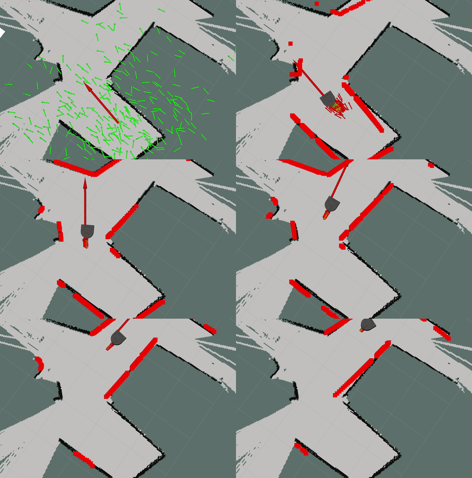
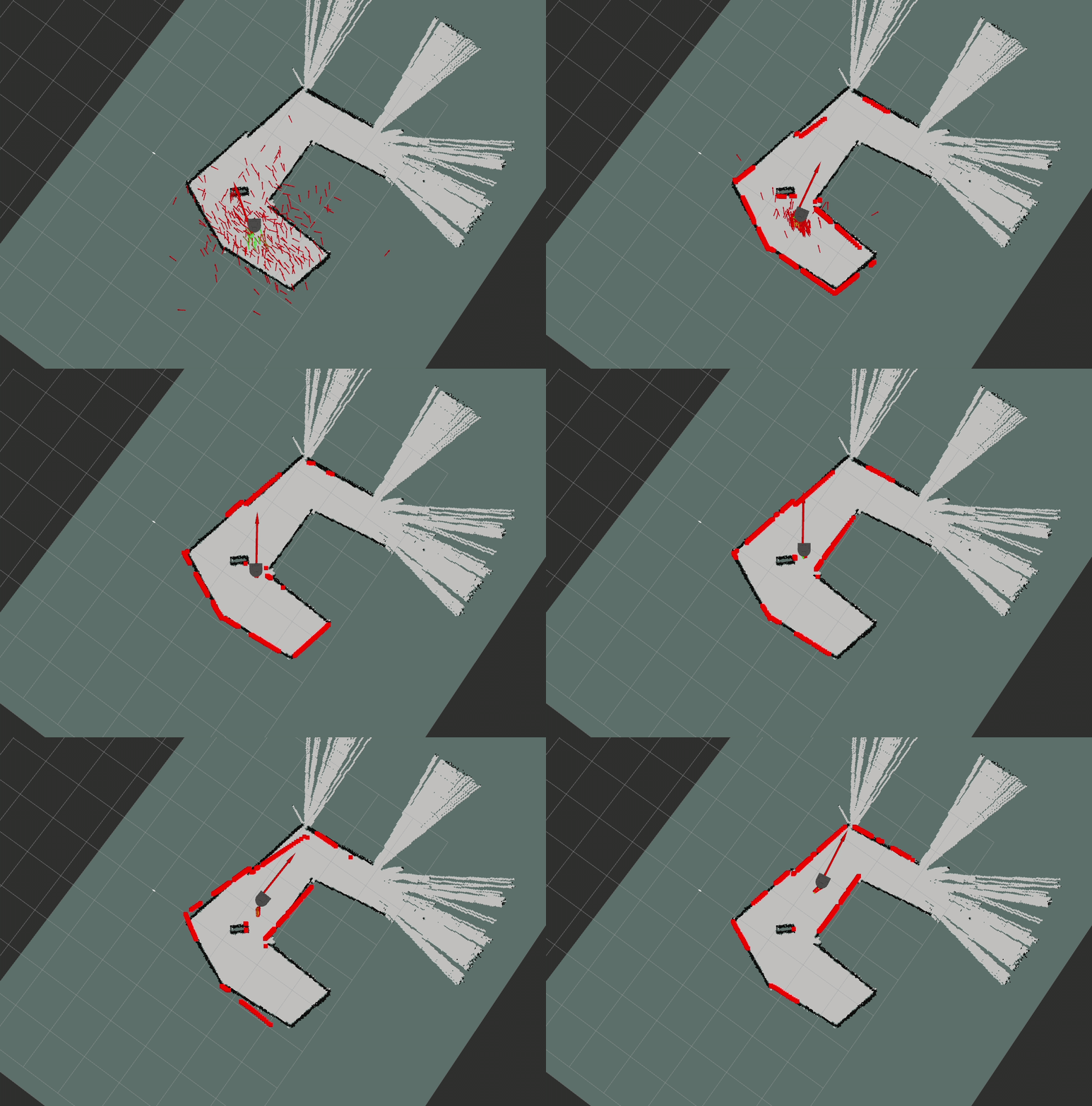
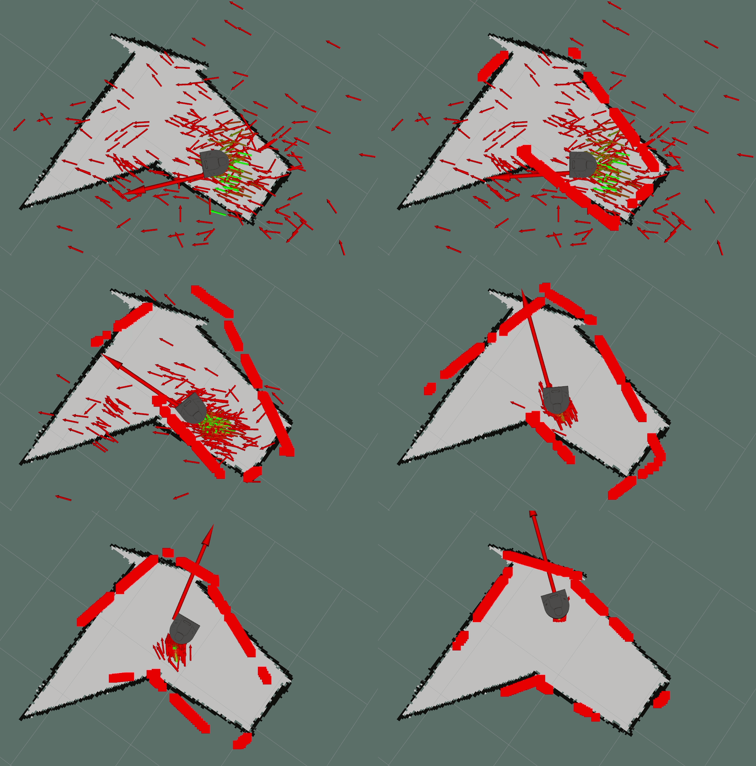
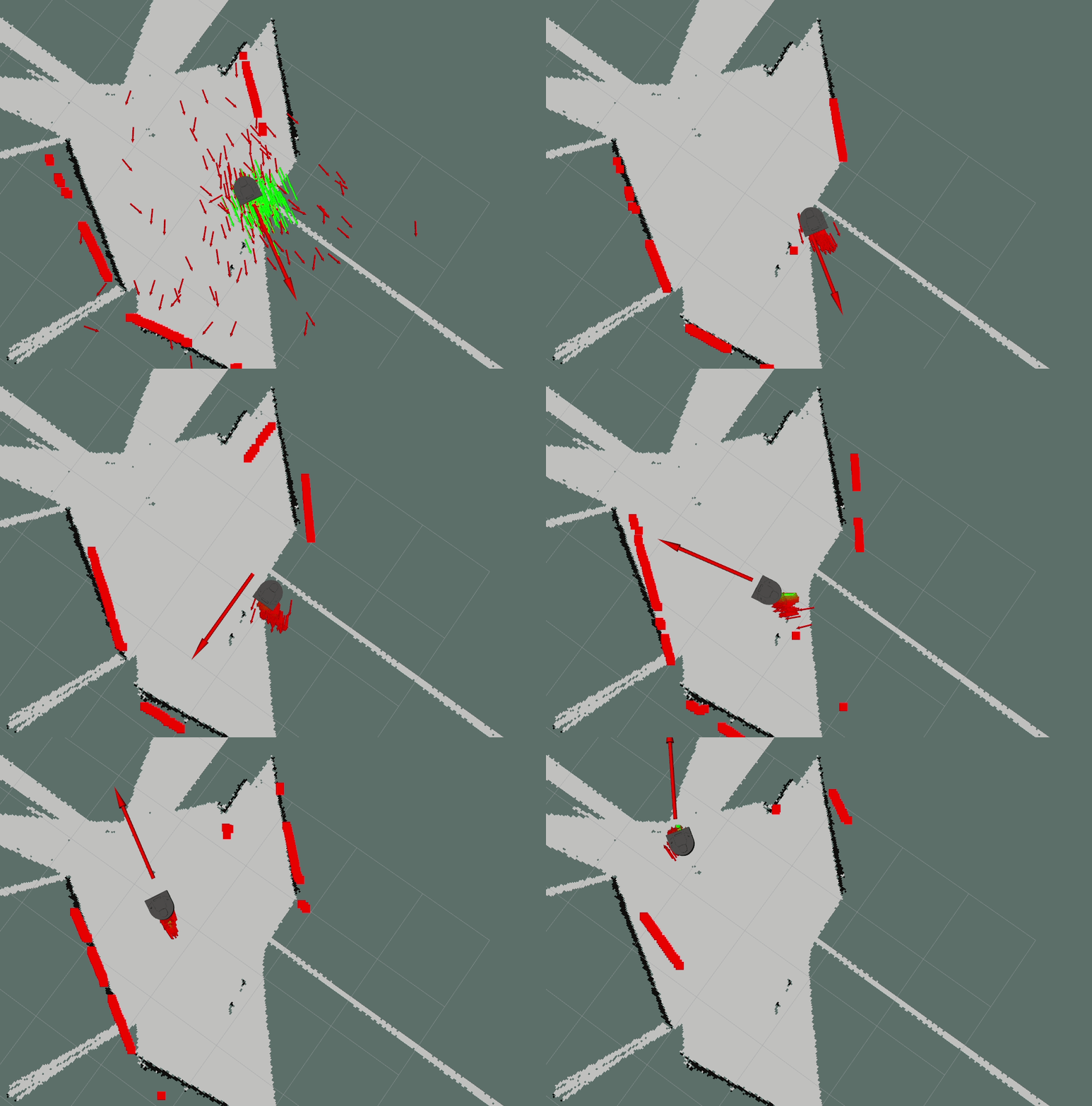
The overall results from testing our particle filter on pre-recorded data can be seen below. Note that the large red arrow represents the “ground truth” (aka the actual position of the robot based on a camera looking at fiducial tags on the ceiling), and the robot represents our filter’s best estimate of the robot’s current position. Each small arrow represents a “hypothesis” of a possible location of the robot, and its color indicates how much we believe in that estimate based on what our lidar is currently seeing (where red = unlikely hypothesis, green = likely hypothesis).

Project Details (excerpt of our write-up)

Project goal

The objective of implementing a Particle Filter is to create a method for figuring out where the robot is within a known map. Although there are mathematically straightforward ways to compute this, there are usually runtime considerations that prevent these from being implemented as-is. In a particle filter, we attempt to compute a “good enough” approximation by tracking and updating a series of poses, which we assign weights to that represent our level of confidence in that particular pose.

What we did

The following steps are implemented in our Particle Filter:

• Create a series of particles with varying positions and poses around our initial estimate (high uncertainty, lots of variation)
• Compute weights for each particle
  • Line up the center of the lidar data with the particle
  • For each point in the lidar, compute what map position that’d be using the following pseudocode:

          x  = particle.x + point_r*cos(point_theta + particle.theta)
          y  = particle.y + point_r*sin(point_theta + particle.theta)
    

  • For each of the projected lidar points, compute the distance to the nearest point in the map + If the projection is off the map, discard the projection
  • Compute the average distance between the projection and the map
  • Create a weight value that is inversely proportional to the distance
• Normalize weights (adjust weights such that their sum equal 1)
• Update most likely robot pose (computed by averaging the x,y, and theta of the top 20 or so particles)
• Resample particles (randomly choose particles from a weighted set, add noise that is proportional to the variance)
• Update particles with the odometry (move all of the particles based on movement reported by the robot’s encoders) using the following pseudocode:

  r = distance(prev_pose, current_pose)
  for each particle in the particle cloud:
        particle.x += r*cos(particle.theta)
        particle.y += r*sin(particle.theta)
  

• Go back to the compute weights step and repeat the process

Full Project Write-up

To read more about this project and to see our full-length project write-up, visit the link below!